dat <- read.csv("https://biostat.ku.dk/PROMS/exampledata.csv")Data analysis summary day 1
Data example: five symptoms in RA patients
| Without Any Difficulty? (0) | With Some Difficulty? (1) | With Much Difficulty? (2) | Unable To Do (3) |
|---|---|---|---|
| □ | □ | □ | □ |
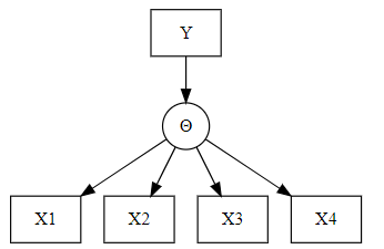
Latent (unobservable) variable \(\Theta\), items \((X_i)_{i\in I}\), categorical exogenous variable \(Y\) (gender, treatment group, age group)
tabulate items
table(dat$it1, useNA = "ifany")
   0    1    2    3 <NA>
71 163 79 80 9 table(dat$it2, useNA = "ifany")
   0    1    2    3 <NA>
123 117 87 64 11 table(dat$it3, useNA = "ifany")
   0    1    2    3 <NA>
45 115 97 136 9 table(dat$it4, useNA = "ifany")
   0    1    2    3 <NA>
41 100 104 150 7 table(dat$it5, useNA = "ifany")
   0    1    2    3 <NA>
 114  131   88   64    5
visualize items
count <- c(table(dat$it1), table(dat$it2), table(dat$it3), table(dat$it4), table(dat$it5))
item <- c(rep("it1", 4), rep("it2", 4), rep("it3", 4), rep("it4", 4), rep("it5", 4))
resp <- c(rep(c(0:3), 5))
data <- data.frame(count, item, resp)
## install.packages("ggplot2", repos="http://cran.rstudio.com/")
library(ggplot2)
ggplot(data, aes(fill=resp, y=count, x=item)) +
  geom_bar(position="fill", stat="identity")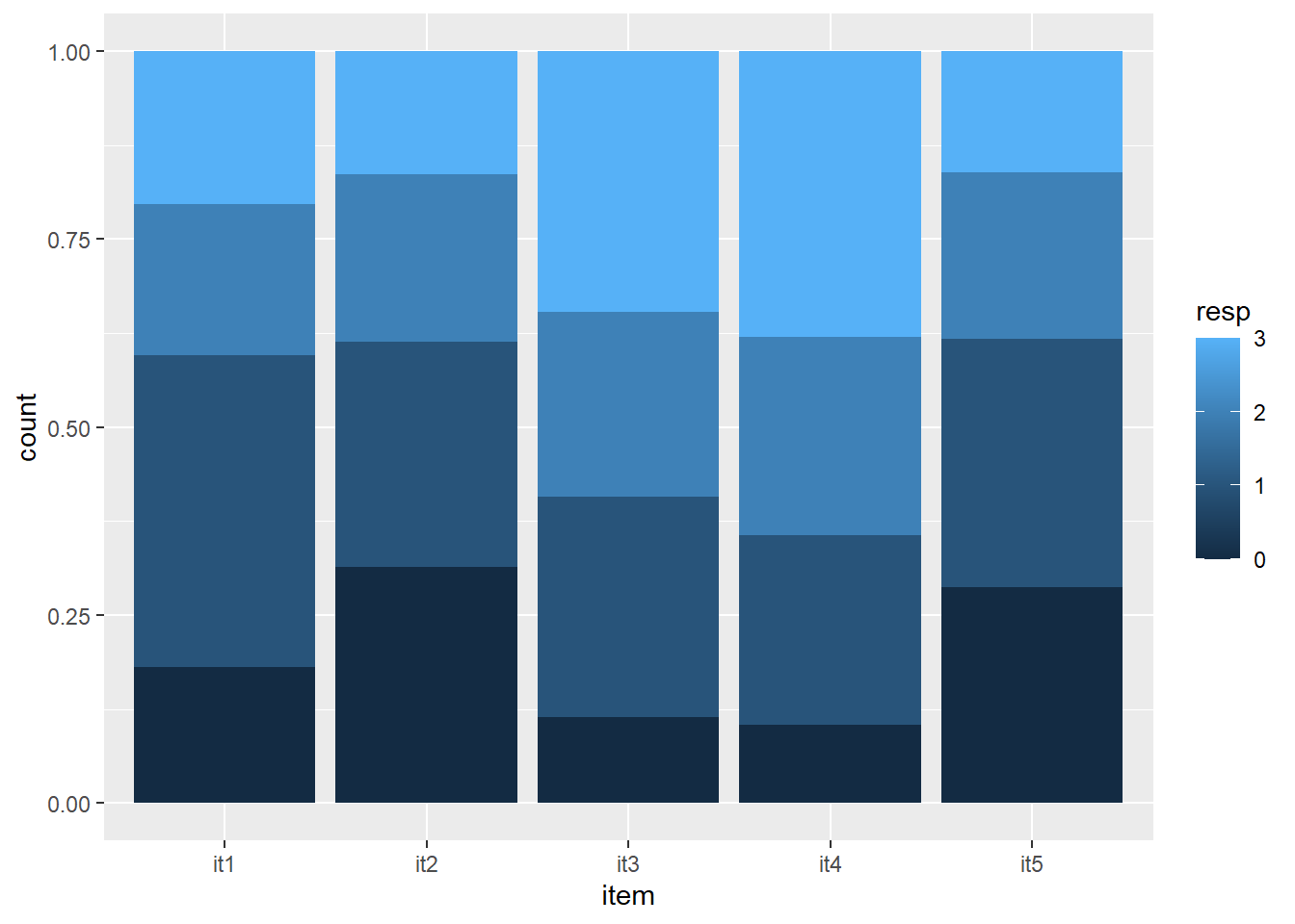
Comparing men and women using the total score
dat$score <- dat$it1 + dat$it2 + dat$it3 + dat$it4 + dat$it5
M <- dat$score[(dat$gender==1)]
W <- dat$score[(dat$gender==2)]
wilcox.test(M,W)
    Wilcoxon rank sum test with continuity correction

data:  M and W
W = 12891, p-value = 0.03381
alternative hypothesis: true location shift is not equal to 0
Graphical illustration of monotonicity
dat$R1 <- dat$it2 + dat$it3 + dat$it4 + dat$it5
qplot(dat$R1, dat$it1, geom = 'smooth', span = 0.95) +
  labs(x = 'rest score', y = 'Item 1') +
  ylim(0, 4)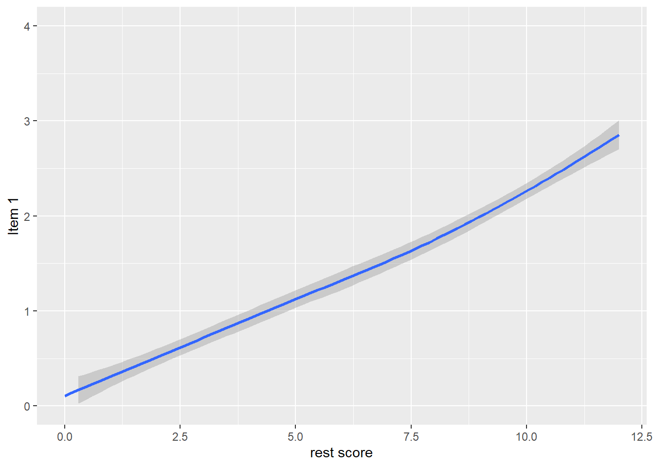
dat$R2 <- dat$it1 + dat$it3 + dat$it4 + dat$it5
qplot(dat$R2, dat$it2, geom = 'smooth', span = 0.95) +
  labs(x = 'rest score', y = 'Item 2') +
  ylim(0, 3)
dat$R3 <- dat$it1 + dat$it2 + dat$it4 + dat$it5
qplot(dat$R3, dat$it3, geom = 'smooth', span = 0.95) +
  labs(x = 'rest score', y = 'Item 3') +
  ylim(0, 3)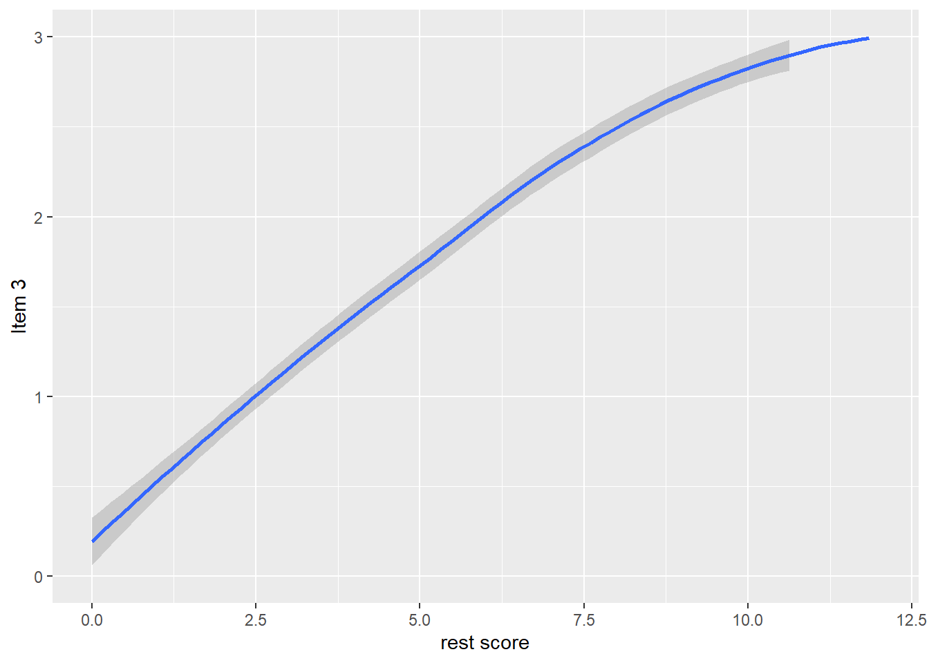
dat$R4 <- dat$it1 + dat$it2 + dat$it3 + dat$it5
qplot(dat$R4, dat$it4, geom = 'smooth', span = 0.95) +
  labs(x = 'rest score', y = 'Item 4') +
  ylim(0, 3)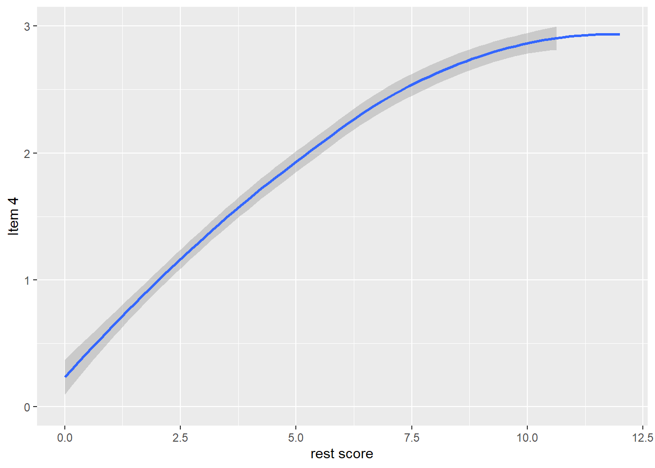
dat$R5 <- dat$it1 + dat$it2 + dat$it3 + dat$it4
qplot(dat$R5, dat$it5, geom = 'smooth', span = 0.95)  +
  labs(x = 'rest score', y = 'Item 5') +
  ylim(0, 3)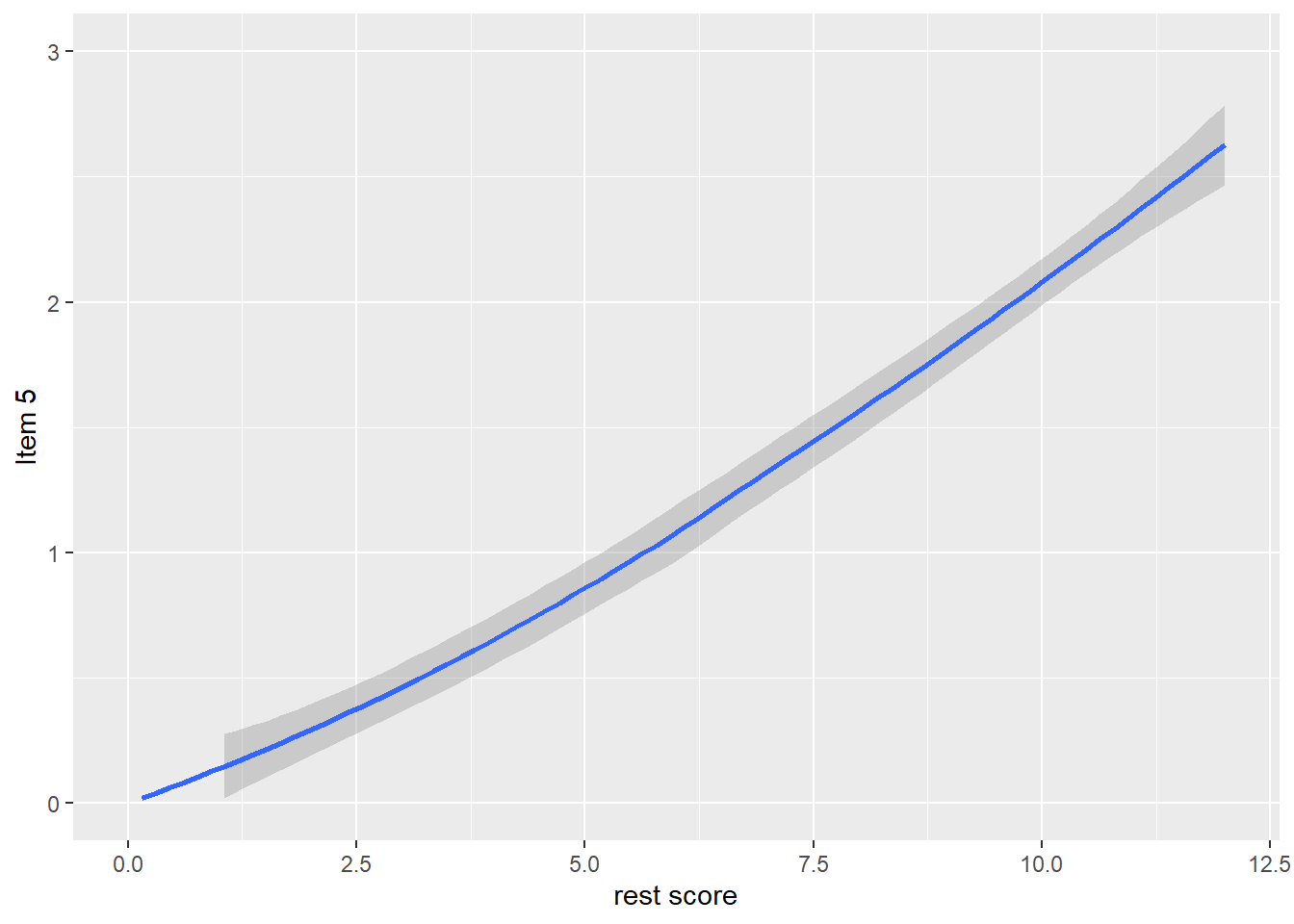
Another graphical illustration of monotonicity
dat$scoregroup <- cut(dat$score, 4)
means <- aggregate(it1 ~ scoregroup, dat, mean)
ggplot(data = means, aes(x = scoregroup, y = it1)) +
  geom_point(size = 3) +
  theme(legend.position = "none") +
  ylim(0, 3)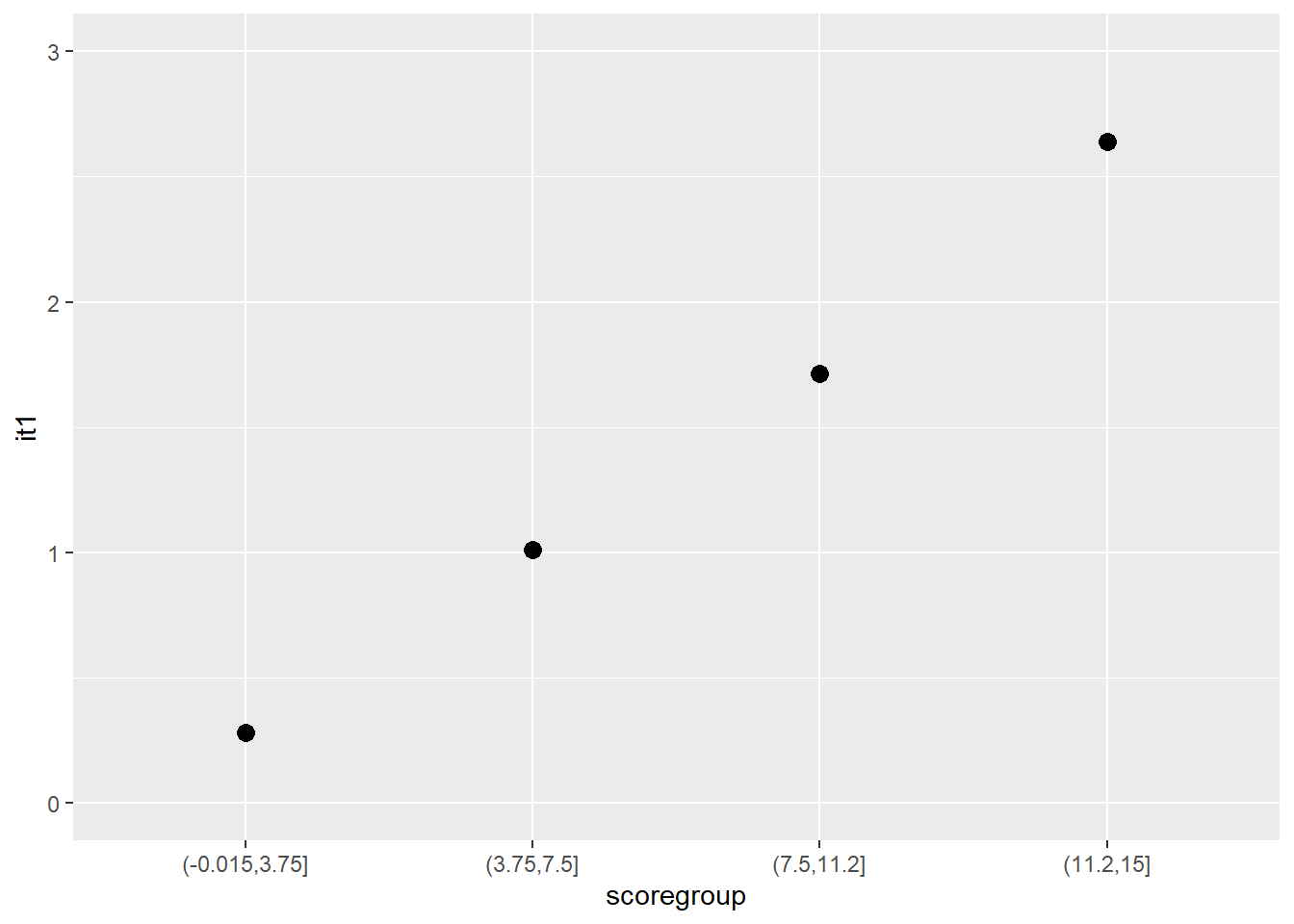
means <- aggregate(it2 ~ scoregroup, dat, mean)
ggplot(data = means, aes(x = scoregroup, y = it2)) +
  geom_point(size = 3) +
  theme(legend.position = "none") +
  ylim(0, 3)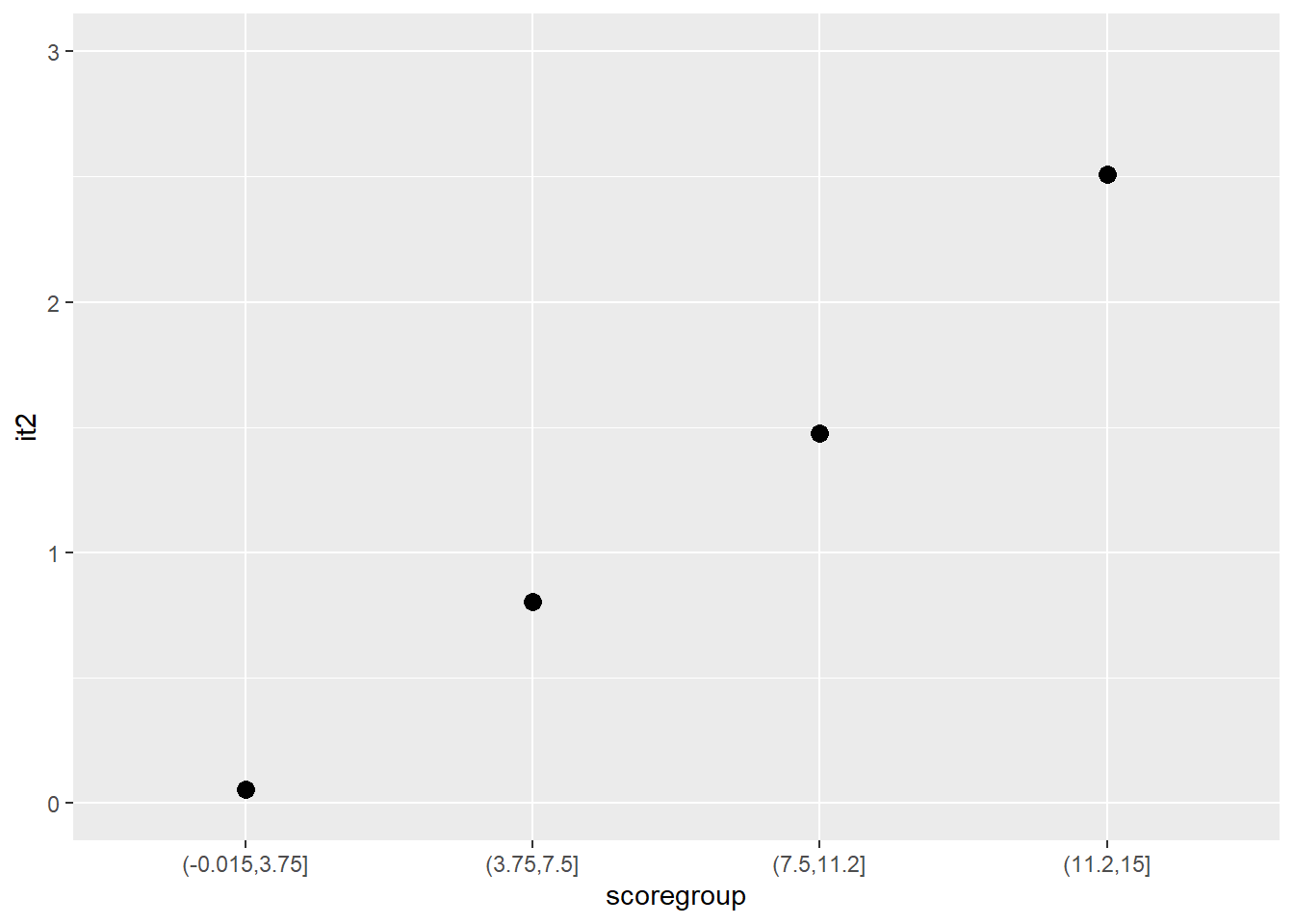
means <- aggregate(it3 ~ scoregroup, dat, mean)
ggplot(data = means, aes(x = scoregroup, y = it3)) +
  geom_point(size = 3) +
  theme(legend.position = "none") +
  ylim(0, 3)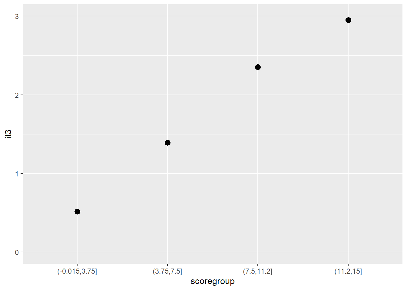
means <- aggregate(it4 ~ scoregroup, dat, mean)
ggplot(data = means, aes(x = scoregroup, y = it4)) +
  geom_point(size = 3) +
  theme(legend.position = "none") +
  ylim(0, 3)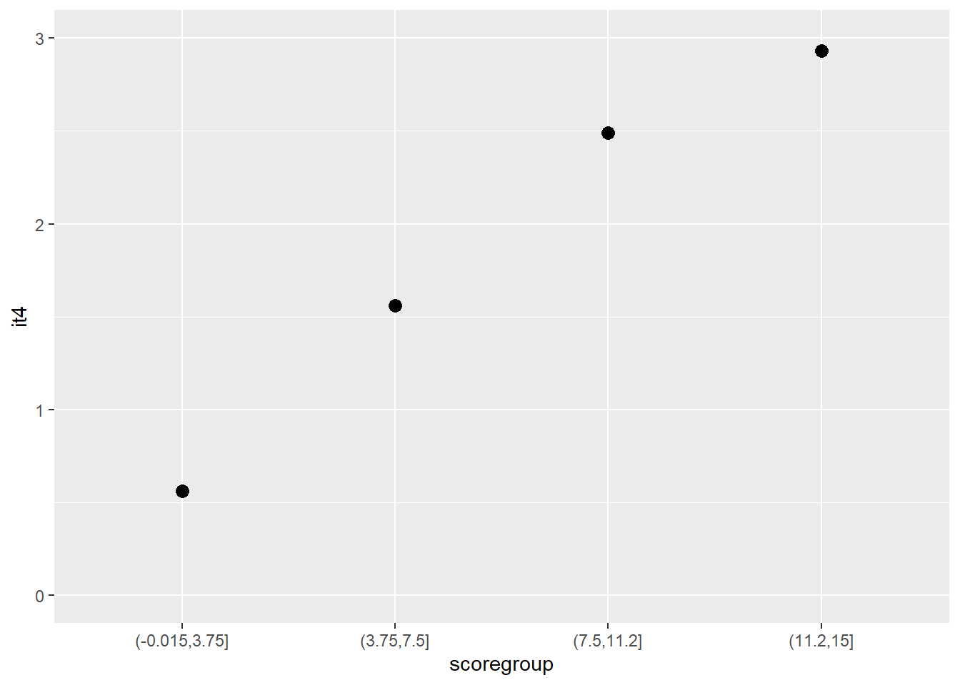
means <- aggregate(it5 ~ scoregroup, dat, mean)
ggplot(data = means, aes(x = scoregroup, y = it5)) +
  geom_point(size = 3) +
  theme(legend.position = "none") +
  ylim(0, 3)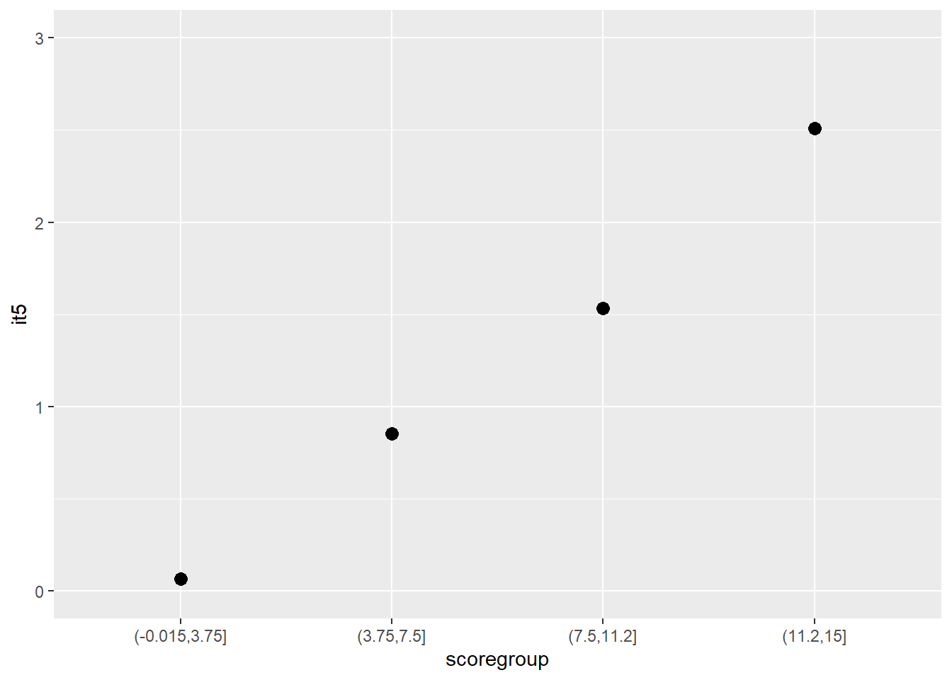
compute inter-item correlations
it <- c("it1", "it2", "it3", "it4", "it5")
correl <- cor(dat[, it], use = "pairwise.complete.obs")
round(correl, 2)
it1 it2 it3 it4 it5
it1 1.00 0.73 0.77 0.74 0.74
it2 0.73 1.00 0.72 0.69 0.73
it3 0.77 0.72 1.00 0.90 0.72
it4 0.74 0.69 0.90 1.00 0.70
it5 0.74 0.73 0.72 0.70 1.00Compute \(\alpha\)
## install.packages("multilevel", repos="http://cran.rstudio.com/")
library(multilevel)
cr <- cronbach(dat[, it])
cr$Alpha
[1] 0.9355742CTT data analysis
Assume that
\[ \begin{bmatrix} x_1\\x_2\\x_3\\x_4\\x_5 \end{bmatrix} \sim N(\mu, \Sigma), \;\;\;\; \mu= \begin{bmatrix} \mu_1\\\mu_2\\\mu_3\\\mu_4\\\mu_5 \end{bmatrix}, \;\;\;\; \Sigma= \begin{bmatrix} \sigma^2_1&\sigma_{12}&\sigma_{13}&\sigma_{14}&\sigma_{15}\\ &\sigma^2_2&\sigma_{23}&\sigma_{24}&\sigma_{25}\\ &&\sigma^2_3&\sigma_{34}&\sigma_{35}\\ &&&\sigma^2_4&\sigma_{45}\\ &&&&\sigma^2_5 \end{bmatrix} \]
X <- dat[, c("it1", "it2", "it3", "it4", "it5")]
mu <- colMeans(X , na.rm = TRUE)
Sigma <- cov(X, use = "pairwise.complete.obs")
Scree plot
X.comp <- X[complete.cases(X), ]
pca <- prcomp(X.comp, scale = TRUE)
eigenvalues <- pca$sdev^2
plot(eigenvalues,
     type = "b",
     xlab = "Principal Component",
     ylab = "Eigenvalue")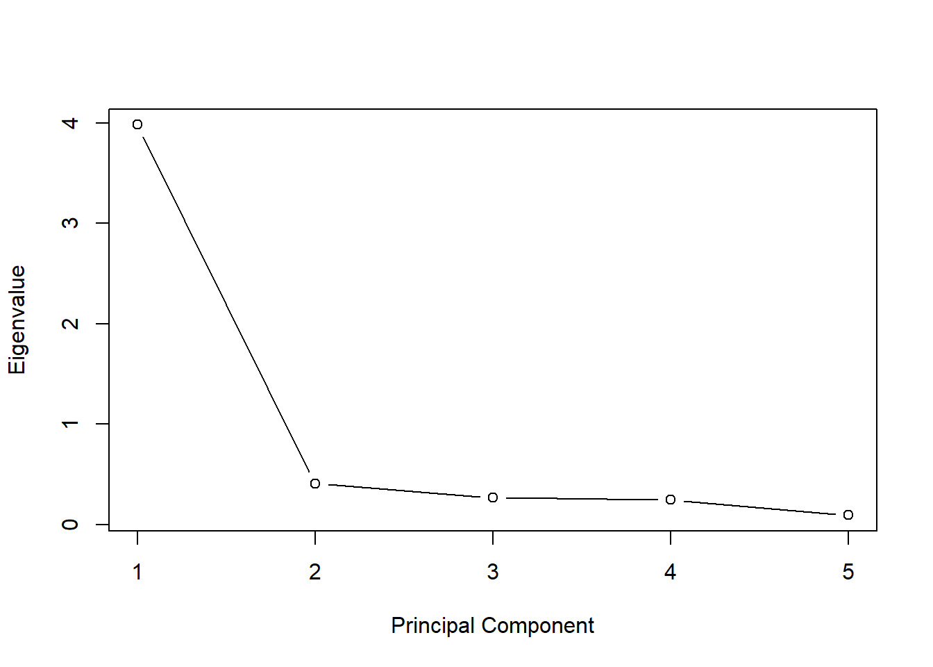
One “factor” explains most of the variation
X.comp <- X[complete.cases(X), ]
pca <- prcomp(X.comp, scale = TRUE)
eigenvalues <- pca$sdev^2
plot(eigenvalues/sum(eigenvalues),
     type = "b",
     xlab = "Principal Component",
     ylab = "Percentage of Variance Explained")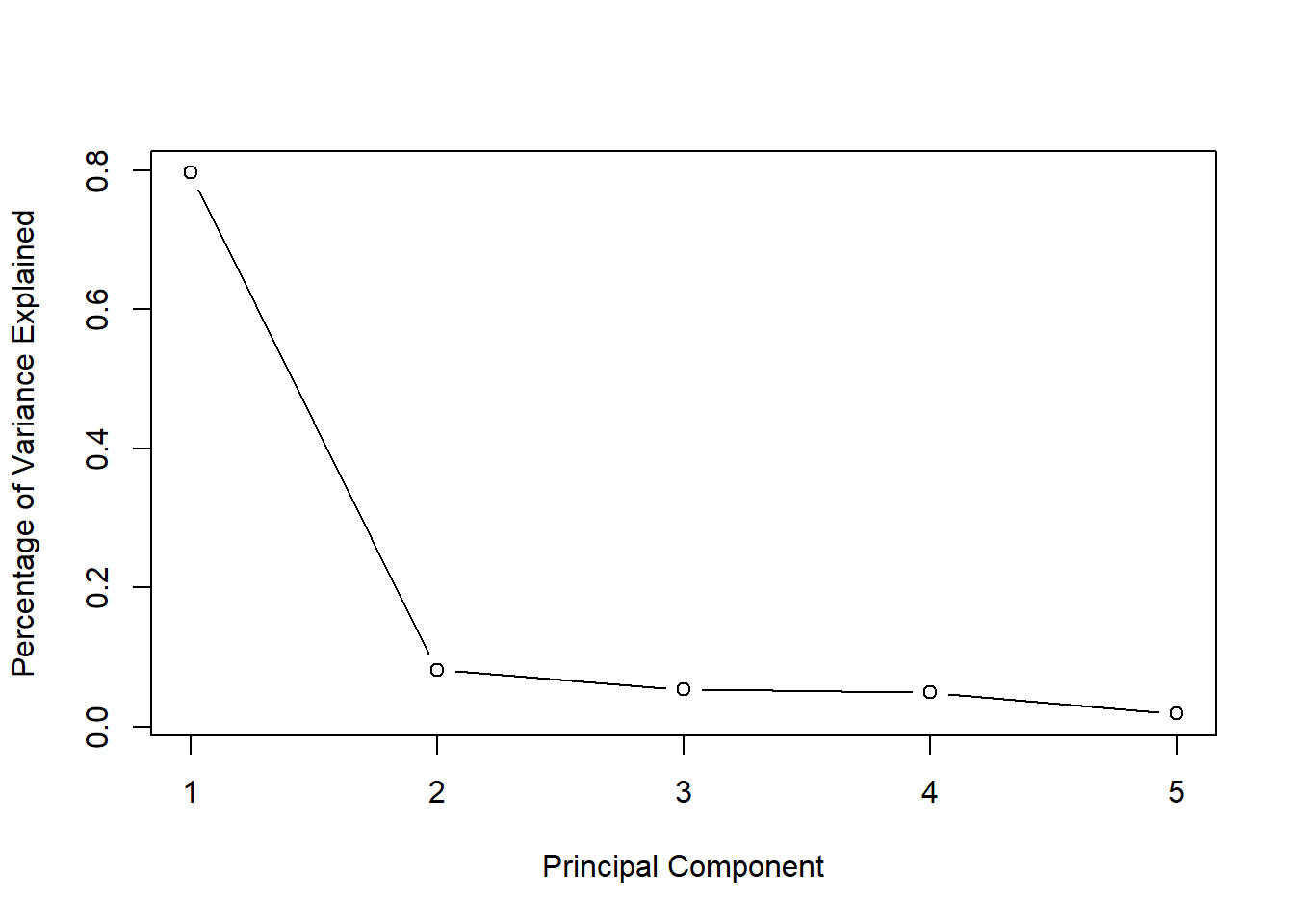
EFA - two factors
\[ \begin{eqnarray} x_{1i} & = & \lambda_{11} f_{1i} + \lambda_{12} f_{2i} + u_{1i} \\ x_{2i} & = & \lambda_{21} f_{1i} + \lambda_{22} f_{2i} + u_{2i} \\ x_{3i} & = & \lambda_{31} f_{1i} + \lambda_{32} f_{2i} + u_{3i} \\ x_{4i} & = & \lambda_{41} f_{1i} + \lambda_{42} f_{2i} + u_{4i} \\ x_{5i} & = & \lambda_{51} f_{1i} + \lambda_{52} f_{2i} + u_{5i} \\ \end{eqnarray} \]
factanal(~ ., data = X, factors = 2, rotation = "none")
Call:
factanal(x = ~., factors = 2, data = X, rotation = "none")

Uniquenesses:
  it1   it2   it3   it4   it5
0.250 0.285 0.017 0.166 0.244

Loadings:
    Factor1 Factor2
it1  0.800   0.331
it2  0.750   0.389
it3  0.990
it4  0.913
it5  0.753   0.435

               Factor1 Factor2
SS loadings      3.583   0.455
Proportion Var   0.717   0.091
Cumulative Var   0.717   0.808

Test of the hypothesis that 2 factors are sufficient.
The chi square statistic is 0.51 on 1 degree of freedom.
The p-value is 0.475
EFA - one factor
\[ \begin{eqnarray} x_{1i} & = & \lambda_{11} f_{1i} + u_{1i} \\ x_{2i} & = & \lambda_{21} f_{1i} + u_{2i} \\ x_{3i} & = & \lambda_{31} f_{1i} + u_{3i} \\ x_{4i} & = & \lambda_{41} f_{1i} + u_{4i} \\ x_{5i} & = & \lambda_{51} f_{1i} + u_{5i} \\ \end{eqnarray} \]
factanal(~ ., data = X, factors = 1, rotation = "none")
Call:
factanal(x = ~., factors = 1, data = X, rotation = "none")

Uniquenesses:
  it1   it2   it3   it4   it5
0.310 0.388 0.099 0.141 0.379

Loadings:
    Factor1
it1 0.831
it2 0.782
it3 0.949
it4 0.927
it5 0.788

               Factor1
SS loadings      3.682
Proportion Var   0.736

Test of the hypothesis that 1 factor is sufficient.
The chi square statistic is 113.21 on 5 degrees of freedom.
The p-value is 8.58e-23
CFA better here because there is a strong theory about the structure:
\[ x_{k,i} = \lambda_{k} f_{1} + u_{k,i}, \;\;\;\;\; (k = 1,2,3,4,5) \]
# install.packages("lavaan")
library(lavaan)
model1 <- 'F1 =~ it1 + it2 + it3 + it4 + it5'
fit <- lavaan::cfa(model = model1, data = X)
This model imposes a structure on the correlation matrix. CFA tests this structure against the observed correlation matrix
library(lavaan)
summary(fit)
lavaan 0.6.17 ended normally after 21 iterations
Estimator ML
Optimization method NLMINB
Number of model parameters 10
Used Total
Number of observations 379 402
Model Test User Model:
Test statistic 114.471
Degrees of freedom 5
P-value (Chi-square) 0.000
Parameter Estimates:
Standard errors Standard
Information Expected
Information saturated (h1) model Structured
Latent Variables:
Estimate Std.Err z-value P(>|z|)
F1 =~
it1 1.000
it2 1.002 0.055 18.165 0.000
it3 1.170 0.047 24.888 0.000
it4 1.136 0.047 23.942 0.000
it5 0.988 0.054 18.367 0.000
Variances:
Estimate Std.Err z-value P(>|z|)
.it1 0.315 0.026 12.219 0.000
.it2 0.447 0.035 12.683 0.000
.it3 0.106 0.015 7.218 0.000
.it4 0.149 0.016 9.159 0.000
.it5 0.418 0.033 12.640 0.000
F1 0.701 0.071 9.849 0.000