Introduction to PROM validation
(ii) recap + data analysis
2024-06-07
Overview
- Recap
- Assumptions/Requirements
- Data example
- Analysis of DIF
Recap
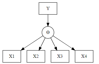
Latent (unobservable) variable \(\Theta\), items \((X_i)_{i\in I}\), categorical exogenous variable \(Y\) (gender, treatment group, age group)
Assumptions/Requirements
Latent (unobservable) variable \(\Theta\), items \((X_i)_{i\in I}\), categorical exogenous variable \(Y\) (gender, treatment group, age group)
Assumptions are (implicitly) made when we combine the items \(X_1,\ldots,X_4\) into a scale
Assumptions/Requirements
- \(\Theta\) unidimensional
Assumptions/Requirements ..
- Monotonous relationship between \(\Theta\) and \(X_i\)
Assumptions/Requirements ..
- Monotonous relationship between \(\Theta\) and \(X_i\)
Assumptions/Requirements ..
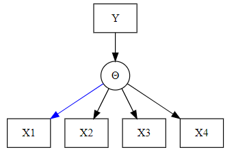
- No differential item functioning (DIF) \(X_i\perp Y|\Theta\)
Assumptions/Requirements ..
- No differential item functioning (DIF) \(X_i\perp Y|\Theta\)
Assumptions/Requirements ..
- Local independence: \(X_i\perp X_j|\Theta\)
Assumptions/Requirements ..
- Local independence: \(X_i\perp X_j|\Theta\)
Requirements/assumptions ..
Requirements/assumptions ..
- .. are testable !
- .. Will discuss how to test them based on observed data.
Requirements/assumptions ..
- .. are testable !
- .. Will discuss how to test them based on observed data.
- Scale is valid \(\Rightarrow\) Assumptions (i)-(iv) are met
- Assumptions (i)-(iv) are not met \(\Rightarrow\) Scale is not valid
Requirements/assumptions ..
- .. are testable !
- .. Will discuss how to test them based on observed data.
- Scale is valid \(\Rightarrow\) Assumptions (i)-(iv) are met
- Assumptions (i)-(iv) are not met \(\Rightarrow\) Scale is not valid
Will use sum score as a proxy for the unobserved \(\Theta\).
Stratified analysis
Differential item functioning (DIF)
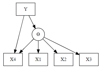
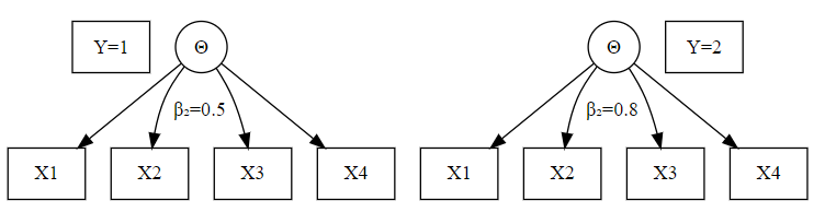
Fundamental assumption: there is no differential item functioning (DIF). Mathematical notation: \[ X_i\perp Y|\Theta \] the item response does not depend directly on a covariate \(Y\) like gender.
Requirement of no DIF
The item response does not depend directly on a covariate \(Y\) like gender.
- It depends only indirectly on a covariate
- Not a problem in a language test if girls score higher than boys on an item
Holland, Wainer. Differential Item Functioning. Differential item functioning. Hillsdale, NJ: Erlbaum, 1993.Requirement of no DIF
The item response does not depend directly on a covariate \(Y\) like gender.
- It depends only indirectly on a covariate
- Not a problem in a language test if girls score higher than boys on an item, but if girls systematically score higher than boys who are at the same level there is something wrong the item.
Holland, Wainer. Differential Item Functioning. Differential item functioning. Hillsdale, NJ: Erlbaum, 1993.Example data
Symptoms in colitis ulcerosa data
Symptoms in colitis ulcerosa data
Symptoms in colitis ulcerosa data
five exogenous variables
interv,status,sex,age,health
Symptoms in colitis ulcerosa data
five exogenous variables
interv,status,sex,age,health
11 symptoms
Anxiety,Anger,Hopeless,Lonely,Restless,Dependen,Tense,Touchy,Shame,Depress,Crying
(3 positive states (Happy, Confiden, Goodhumo)).
Example data. Visualize
Example data. Visualize
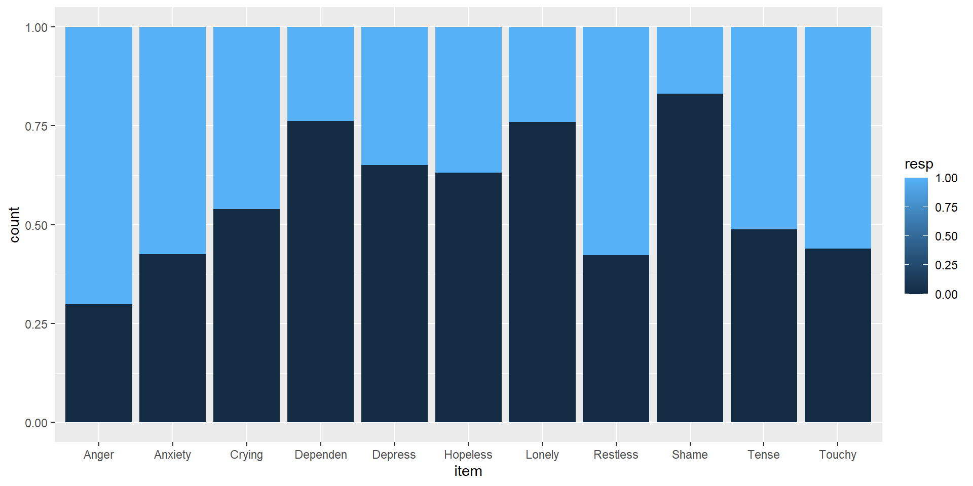
Symptom scale example, patients
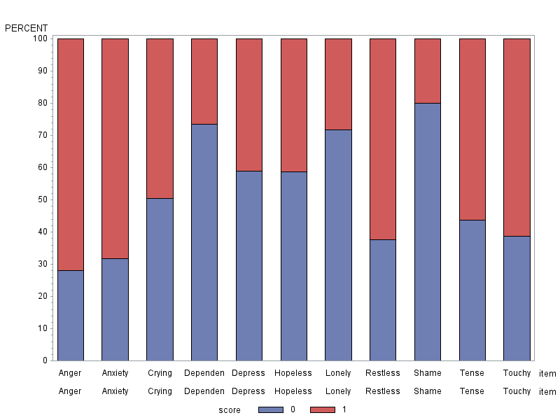
Symptom scale example, controls
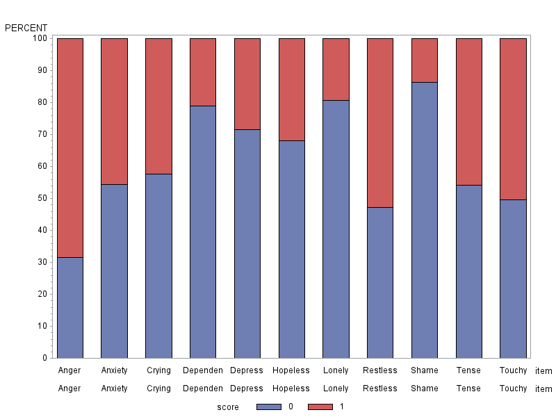
Symptom scale example
It seems that the item Anxiety sticks out. Indeed patients and control differ significantly wrt. the item anxiety. Can test this
- OR, Mantel-Häentzel
- partial correlation
- (ordinal) logistic regression
Holland, Thayer. Differential item performance and the Mantel-Haenszel procedure. In Wainer & Braun (Eds.), Test Validity (pp. 129-145). Hillsdale, NJ: Erlbaum, 1988Swaminathan, Rogers. Swaminathan, Rogers, 1990. Jornal of Educational Measurement, 27, 361-370, 1990.DIF can be visualized
Partial correlation
Partial correlation measures the degree of association between two random variables, with the effect of a set of controlling random variables removed
Can be used to explain (some of) the correlation between \(X\) and \(Y\). We can test if \(Z\) explains all of the correlation between \(X\) and \(Y\)
Partial correlation
Partial correlation measures the degree of association between two random variables, with the effect of a set of controlling random variables removed
\[ \hat{\rho}_{XY\cdot\mathbf{Z}}=\frac{N\sum_i r_{X,i}r_{Y,i}-\sum_i r_{X,i}\sum_i r_{Y,i}} {\sqrt{N\sum_i r_{X,i}^2-\left(\sum_i r_{X,i}\right)^2}~\sqrt{N\sum_i r_{Y,i}^2-\left(\sum_i r_{Y,i}\right)^2}} \]
Can be used to explain (some of) the correlation between \(X\) and \(Y\). We can test if \(Z\) explains all of the correlation between \(X\) and \(Y\)
Alternative illustration
Stratified analysis
DIF example
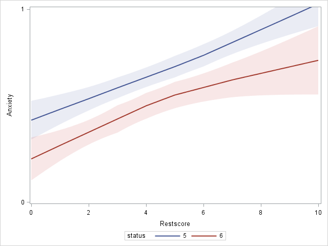
gender = \(Y\). We’ll look at three items Crying, Anger, Hopeless.
DIF example
gender = \(Y\). We’ll look at three items Crying, Anger, Hopeless.
- Marginal association: correlation \(X_i\sim Y\)
- Conditional association: partial correlation \(X_i\sim Y|\)
score
DIF example, Crying
Marginal association - correlation \(X_i\sim Y\)
DIF example, Crying
Marginal association - correlation \(X_i\sim Y\)
         cor
3.385557e-01 8.678151e-19 Partial correlation \(X_i\sim Y|\)score
DIF example, Crying
Marginal association - correlation \(X_i\sim Y\)
         cor
3.385557e-01 8.678151e-19
Partial correlation \(X_i\sim Y|\)score
Code
   estimate      p.value
1 0.1547597 7.927312e-05
DIF example, Anger
Marginal association - correlation \(X_i\sim Y\)
DIF example, Anger
Marginal association - correlation \(X_i\sim Y\)
         cor
0.1448186591 0.0002214976 partial correlation \(X_i\sim Y|\)score
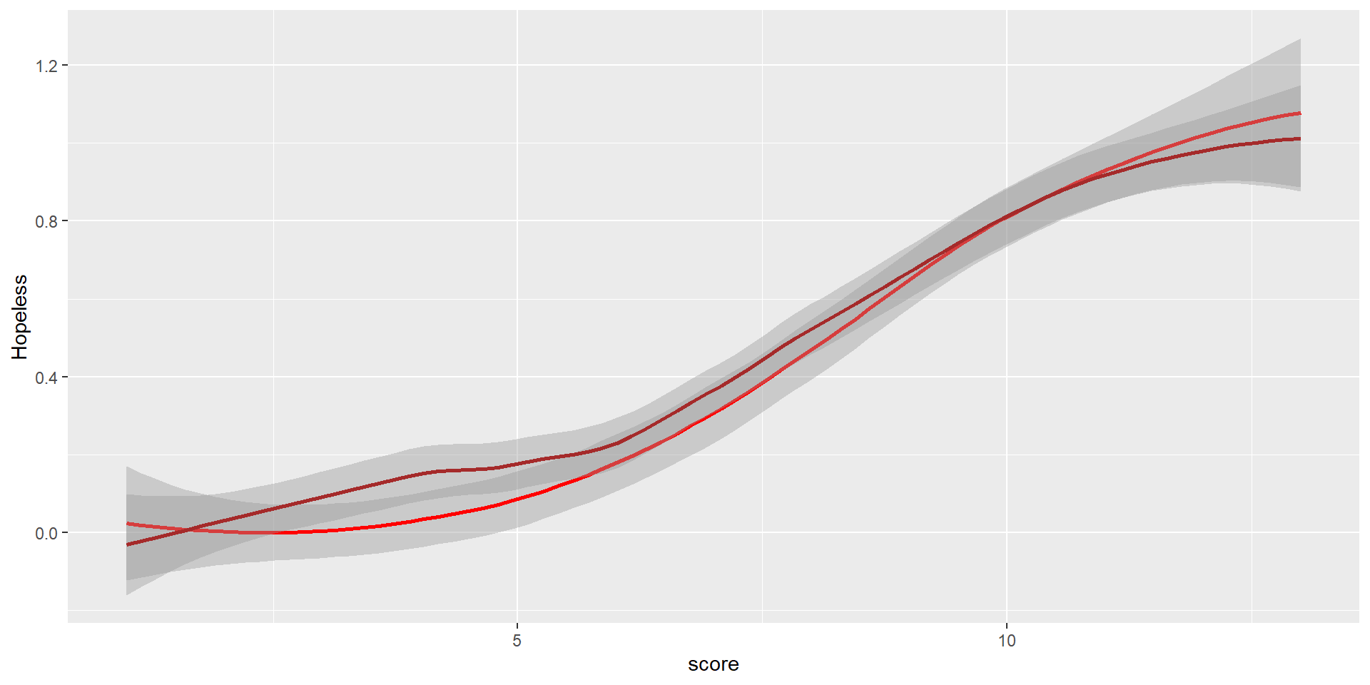
DIF example, Hopeless
Marginal association - correlation \(X_i\sim Y\)
DIF example, Hopeless
Marginal association - correlation \(X_i\sim Y\)
         cor
0.1340163752 0.0006376999 partial correlation \(X_i\sim Y|\)score
Visualize DIF
Local dependence (LD)
- \(\Theta\) unidimensional
- Monotonous relationship \(\Theta\sim X_i\)
- No DIF \(X_i\perp Y|\Theta\)
- (iv) Local independence: \(X_i\perp X_j|\Theta\)
Local independence = absence of LD
- technical assumption not as intuitive as (i)-(iii)
LD
Intuition
- Those with a low level of \(\theta\) will tend to score low on all items
- Those with a high level of \(\theta\) will tend to score high on all items
- Items are correlated because they all depend on \(\theta\)
- It is relatively new to think about local dependence in terms of response dependence.
History
Lord (1980, section 2.4):
- “local independence ..
Heinen (1996, p.7):
- “.. literature on latent trait models ..
History
Lord (1980, section 2.4):
- “local independence .. follows automatically from unidimensionality. It is not an additional assumption”
Heinen (1996, p.7):
- “.. literature on latent trait models .. inclined to define local independence as a special case of unidimensionality”
History
Lord (1980, section 2.4):
- “local independence .. follows automatically from unidimensionality. It is not an additional assumption”
Heinen (1996, p.7):
- “.. literature on latent trait models .. inclined to define local independence as a special case of unidimensionality”
Lord, F. M. (1980). Applications of Item Response Theory to Practical Testing Problems. Erlbaum Associates.
Heinen, T. (1996). Latent class and discrete latent trait models: Similarities and differences. Thousand Oaks, CA: Sage.
Similar to DIF
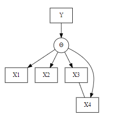
Looking at the graph
it reminds us of the test for DIF.
Similar to DIF
So if we forget for a moment that \(X_4\) is an item and think of it as an exogenous variable like gender we can handle this as a DIF problem. Then the score is \[ R_4=X_1+X_2+X_3 \] and we test conditional independence \[ X_3\perp X_4|R_4 \]
Similar to DIF
Similar argument where \(X_3\) and \(X_4\) switch places tells us that computing the rest score \(R_3=X_1+X_2+X_4\) and testing
\[ X_3\perp X_4|R_3 \]