Introduction to PROM validation
Data analysis crash course
- today: intro (data set, notation, ..), consistency, reliability (Cronbachs \(\alpha\)), invariance (DIF), local dependence, criterion validity
- also today: CFA
- after today: video lectures (examples in SAS and R), exercises on Absalon, ask question by e-mail to
kach@sund.ku.dk - next time: Q & A, work on the exam together
Intro
- data set (Exercise Adherence Rating Scale; EARS)
- path diagrams
Exercise Adherence Rating Scale (EARS)
measuring adherence to prescribed home exercise
FILENAME preg URL "http://publicifsv.sund.ku.dk/~kach/scaleval/EARS.csv";
PROC IMPORT FILE=preg OUT=SASUSER.EARS DBMS=csv REPLACE;
GETNAMES=YES;
DELIMITER=';';
RUN;
https://www.sciencedirect.com/science/article/pii/S0031940616304801
Exercise Adherence Rating Scale (EARS)
measuring adherence to prescribed home exercise
https://www.sciencedirect.com/science/article/pii/S0031940616304801
Notation
Association between the variables \(A\) and \(B\) - and we believe that \(A\) causes \(B\). We put boxes around observed (manifest) variables
Notation
We put circles around unobserved (latent) variables. Will use \(\Theta\) or \(\theta\) (greek letter “theta”) to indicate latent variables.
Exercise Adherence Rating Scale (EARS)
Latent (unobservable) variable \(\Theta\), items \((X_i)_{i\in I}\), categorical exogenous variables \(Y\) (gender, age group)
SAS macro %itemmarg.sas()
FILENAME im URL 'https://raw.githubusercontent.com/KarlBangChristensen/itemmarg/master/itemmarg.sas';
%include im;
%ITEMMARG(DATA=SASUSER.EARS, ITEMS=item1-item6);
SAS macro %itemmarg.sas()
BARplot R function
Install package (only do this once)
load package and plot
BARplot R function
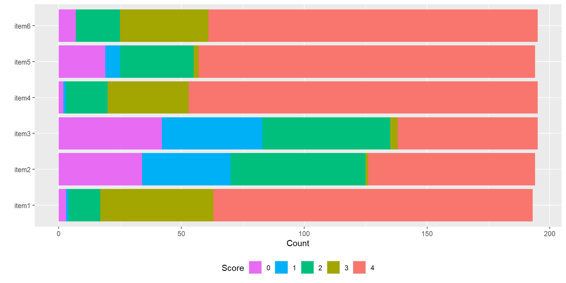
Consistency
items positively correlated because they all measure \(\theta\)
positive association with sum score (proxy for \(\theta\))
many different correlations exist
Polychoric correlation

Metsämuuronen, Front. Appl. Math. Stat., Sec. Statistics and Probability, Volume 8 - 2022 https://doi.org/10.3389/fams.2022.914932, Figure 1.
Inter-item correlations, SAS
| Polychoric Correlations | ||||||||
|---|---|---|---|---|---|---|---|---|
| Variable | With Variable | N | Correlation | Wald Test | LR Test | |||
|
Standard Error |
Chi-Square | Pr > ChiSq | Chi-Square | Pr > ChiSq | ||||
| item1 | item2 | 192 | 0.44618 | 0.08031 | 30.8664 | <.0001 | 23.0330 | <.0001 |
Inter-item correlations, R
Polychoric Correlation, ML est. = 0.4464 (0.0812)
Test of bivariate normality: Chisquare = 43.66, df = 15, p = 0.0001241

  Row Thresholds
  Threshold Std.Err.
1    -2.128  0.23080
2    -1.999  0.20420
3    -1.337  0.12550
4    -0.460  0.09386


  Column Thresholds
  Threshold Std.Err.
1   -0.9340  0.10560
2   -0.3552  0.09233
3    0.3530  0.09256
4    0.3668  0.09275
Inter-item correlations
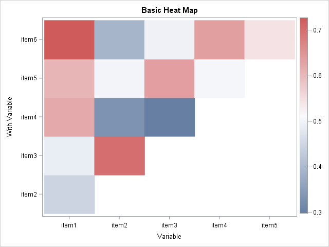
Theoretical model
what we observe
Inter-item correlations, SAS
filename PMH URL "https://raw.githubusercontent.com/KarlBangChristensen/PolyHeatMap/master/PolyHeatMap.sas";
%include PMH;
%PolyHeatMap(dat=SASUSER.EARS, var=item1-item6);
Inter-item correlations, SAS
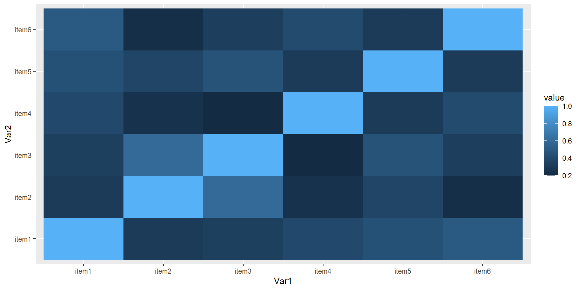
Inter-item correlations, R
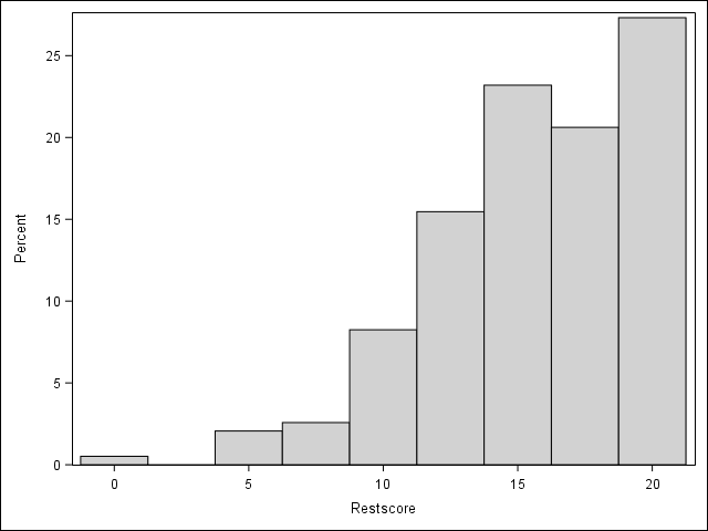
Total score
DATA WORK.EARS;
    SET SASUSER.EARS;
    score=SUM(OF item1-item6);
RUN;
PROC SGPLOT DATA=WORK.EARS;
    HISTOGRAM score;
    DENSITY score / TYPE=KERNEL;
RUN;Add item-total correlations, SAS
FILENAME st URL 'https://raw.githubusercontent.com/KarlBangChristensen/scaletest/master/scaletest.sas';
%INCLUDE st;
data WORK.new(where=(nm=0));
    set SASUSER.EARS;
    nm=nmiss(of item1-item6);
run;
%scaletest(data=WORK.new, ncat=5, items=item1-item6, type=SPEARMAN);
Add item-total correlations, SAS
| name | mean | SD | _min | _max | floor | ceiling | Item | total |
|---|---|---|---|---|---|---|---|---|
| item1 | 3.55 | 0.78 | 0.36 | 0.61 | 1.6 | 67.4 | item1 | 0.65 |
| item2 | 2.17 | 1.51 | 0.26 | 0.60 | 17.5 | 35.1 | item2 | 0.76 |
| item3 | 1.96 | 1.51 | 0.22 | 0.60 | 21.5 | 29.2 | item3 | 0.79 |
| item4 | 3.60 | 0.76 | 0.22 | 0.50 | 1.0 | 72.8 | item4 | 0.53 |
| item5 | 3.20 | 1.36 | 0.36 | 0.46 | 9.8 | 70.6 | item5 | 0.72 |
| item6 | 3.49 | 0.93 | 0.32 | 0.61 | 3.6 | . | item6 | 0.66 |
Add item-total correlations, R
library(devtools)
gh <- "https://raw.githubusercontent.com/KarlBangChristensen/scaletest/master/scaletest.R"
source_url(gh)
scaletest(data = items, min_item_score = 0, max_item_score = 4)
mean sd floor ceiling min max item_score_corr
item1 3.549223 0.7765522 1.554404 67.35751 0.3015623 0.4983621 0.6502836
item2 2.170103 1.5088454 17.525773 35.05155 0.2316051 0.5982678 0.7306689
item3 1.958974 1.5054400 21.538462 29.23077 0.2075063 0.5982678 0.7791156
item4 3.600000 0.7557341 1.025641 72.82051 0.2075063 0.4315206 0.5486745
item5 3.195876 1.3553897 9.793814 70.61856 0.3371068 0.4623874 0.7403411
item6 3.487179 0.9325664 3.589744 68.71795 0.2316051 0.4983621 0.6199170
raw_corr
item1 0.5393439
item2 0.5240605
item3 0.5987229
item4 0.4252349
item5 0.5650794
item6 0.4784750Visualizing item-total correlation
ods graphics on;
ods html5 style=htmlblue;
options nonotes;
DATA WORK.EARS;
    SET SASUSER.EARS;
    score=SUM(OF item1-item6);
RUN;
PROC RANK data=WORK.EARS out=WORK.grouped groups=5;
    VAR score;
    RANKS scoregroup;
RUN;
PROC MEANS DATA=WORK.grouped;
    VAR item1;
    CLASS scoregroup;
    OUTPUT OUT=item1means MEAN=m LCLM=l UCLM=u;
RUN;
PROC SGPLOT DATA=WORK.item1means;
    BAND X=scoregroup LOWER=l UPPER=u / LEGENDLABEL='95% CI';
    SERIES X=scoregroup Y=m;
    LABEL m='Mean score on anxiety item';
RUN;| Analysis Variable : item1 | ||||||
|---|---|---|---|---|---|---|
| Rank for Variable score | N Obs | N | Mean | Std Dev | Minimum | Maximum |
| 0 | 38 | 36 | 2.8333333 | 1.1084094 | 0 | 4.0000000 |
| 1 | 41 | 41 | 3.1951220 | 0.7489831 | 1.0000000 | 4.0000000 |
| 2 | 29 | 29 | 3.6551724 | 0.4837253 | 3.0000000 | 4.0000000 |
| 3 | 46 | 46 | 3.9565217 | 0.2948839 | 2.0000000 | 4.0000000 |
| 4 | 41 | 41 | 4.0000000 | 0 | 4.0000000 | 4.0000000 |
Reliability
\(\alpha\) is a measure of
- consistency: inter-item correlations positive ?
- reliability: how precisely does the score measure \(\theta\) ?
compute \(\alpha\), SAS
PROC CORR DATA=SASUSER.EARS ALPHA NOMISS;
    VAR item1-item6;
    ODS SELECT "Cronbach Coefficient Alpha";
RUN;\(\alpha\), SAS
| Cronbach Coefficient Alpha | |
|---|---|
| Variables | Alpha |
| Raw | 0.755560 |
| Standardized | 0.774217 |
compute \(\alpha\), R
only do this once
install.packages("multilevel", repos="http://cran.rstudio.com/")compute \(\alpha\)
\(\alpha\)
is a lower boundary of the reliability
\(\alpha\)
is a lower boundary of the reliability, but only if items are unidimensional and there is no local dependence.
\(\alpha\)
is a lower boundary of the reliability, but only if items are unidimensional and there is no local dependence. It is not a measure of validity.
Invariance (no differential item functioning; DIF)
Notation
\[ X_i\perp Y|\Theta \]
the item response does not depend directly on a covariate \(Y\)
Covariate
the covariate long groups respondents in two groups.
- an association between
longand an item should only occur because of an association betweenlongand the latent variable.
Correlation ..
.. measures the degree of association between two random variables \(X\) and \(Y\)
Partial correlation
.. measures the degree of association between \(X\) and \(Y\), with the of a controlling variable \(Y\) removed
\[ \hat{\rho}_{XY\cdot\mathbf{Z}}=\frac{N\sum_{i=1}^N r_{X,i}r_{Y,i}-\sum_{i=1}^N r_{X,i}\sum_{i=1}^N r_{Y,i}} {\sqrt{N\sum_{i=1}^N r_{X,i}^2-\left(\sum_{i=1}^N r_{X,i}\right)^2}~\sqrt{N\sum_{i=1}^N r_{Y,i}^2-\left(\sum_{i=1}^N r_{Y,i}\right)^2}} \]
Can be used to explain (some of) the correlation between \(X\) and \(Y\). We can test if \(Z\) explains all of the correlation between \(X\) and \(Y\)
Correlation and partial correlation
Correlation and partial correlation
Correlation
| Spearman Correlation Statistics (Fisher's z Transformation) | |||||||||
|---|---|---|---|---|---|---|---|---|---|
| Variable | With Variable | N | Sample Correlation | Fisher's z | Bias Adjustment | Correlation Estimate | 95% Confidence Limits |
p Value for H0:Rho=0 |
|
| item2 | long | 162 | -0.19229 | -0.19472 | -0.0005972 | -0.19172 | -0.335979 | -0.038663 | 0.0141 |
this is not evidence that something is wrong with the item
Partial correlation
| Spearman Partial Correlation Statistics (Fisher's z Transformation) | ||||||||||
|---|---|---|---|---|---|---|---|---|---|---|
| Variable | With Variable | N | N Partialled | Sample Correlation | Fisher's z | Bias Adjustment | Correlation Estimate | 95% Confidence Limits |
p Value for H0: Partial Rho=0 |
|
| item2 | long | 162 | 1 | -0.17629 | -0.17815 | -0.0005509 | -0.17575 | -0.321684 | -0.021668 | 0.0251 |
members of the two groups with the same total score differ significantly so there is a problem with the item.
DIF can be visualized
DIF can be visualized
DIF can be visualized
DIF can be visualized
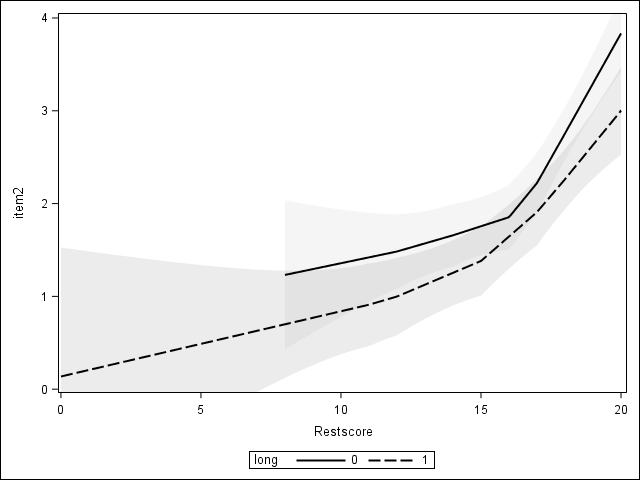
Looking for DIF
Test DIF using
- Mantel-Haenszel
- Partial correlation
- Logistic regression
Local dependence
Four testable assumption - three ((i), (ii), and (iii)) are intuitive. However (iv) local independence is a technical assumption and it is not as intuitive.
(iv) local independence
trick
think of \(X_4\) as an exogenous variable and handle this as a DIF problem.
- score is \(R_4=X_1+X_2+X_3\)
- we test conditional independence \(X_3\perp X_4|R_4\)
trick
a similar argument where \(X_3\) and \(X_4\) switch places
- compute (rest) score \(R_3=X_1+X_2+X_4\)
- test \(X_3\perp X_4|R_3\)
Tjur (1982). Scandinavian Journal of Statistics, 9, 23–30. http://www.jstor.org/stable/4615850
SAS macro
FILENAME TJUR URL 'http://192.38.117.59/~kach/macro/tjur.sas';
%INCLUDE TJUR;
DATA WORK.nm;
  SET SASUSER.EARS;
  IF NMISS(OF item1-item6)>0 THEN DELETE;
RUN;
%TJUR(DATA=WORK.nm, ITEMS=item1-item6);
PROC PRINT DATA=TJUR NOOBS;
  WHERE _TYPE_='CORR';
  VAR _name_ item1-item6;
  FORMAT item1-item6 8.2;
RUN;
Local dependence in EARS data
15 item pairs (two partial correlations for each of them).
let’s focus
| item1 | item2 | item3 | item4 | item5 | item6 | |
|---|---|---|---|---|---|---|
| item1 | 1.00 | |||||
| item2 | 1.00 | 0.29 | ||||
| item3 | 0.35 | 1.00 | ||||
| item4 | 1.00 | |||||
| item5 | 1.00 | |||||
| item6 | 0.01 |
Using R
Read data and calculate rest scores
EARS <- read.csv(url("http://publicifsv.sund.ku.dk/~kach/scaleval/EARS.csv"), sep=';')
items <- EARS[,c("item1","item2","item3","item4","item5","item6")]
nm <- items[complete.cases(items),]
nm$rscore1 <-            nm$item2 + nm$item3 + nm$item4 + nm$item5 + nm$item6
nm$rscore2 <- nm$item1 +            nm$item3 + nm$item4 + nm$item5 + nm$item6
nm$rscore3 <- nm$item1 + nm$item2 +            nm$item4 + nm$item5 + nm$item6
Using R
calculate (some of) the partial correlations
[1] 0.35[1] 0.29Criterion validity
- latent variable \(\Theta\)
score=item1+ … +item6indirect measure of \(\Theta\)- for any variable \(Z\) where \[\textrm{corr}(Z,\Theta)>0\] we expect \(\textrm{corr}(Z,\)
score\()>0\) - This can be tested
Confirmatory factor analysis (CFA) ..
.. is essentially a statistical model that incorporates all the assumptions we have discussed.
- Testing the fit of a CFA model to your data will tell you if the instrument is valid
Two types of factor analysis
Exploratory factor analysis (EFA):
Data is explored to determine the number of underlying factors. Prior knowledge about data generating mechanisms is ignored. Will not be considered here.Confirmatory factor analysis (CFA): Based on prior knowledge a factor structure is postulated and tested against data.
Methods originally developed for continuous items and an assumption of multivariate normal distribution.
CFA model for EARS data
Statistical model for the joint distribution of all items and covariates
CFA model
Statistical model for the joint distribution of all items and covariates
- Allows inclusion of DIF and local dependence
- (Allows models with a multivariate latent variable)
- Builds on the normal distribution
CFA model
SAS procedure CALIS. Hatcher, 1996, doi:10.1080/10705519609540037
R package
lavaan. Rosseel, 2012. doi: 10.18637/jss.v048.i02. http://lavaan.ugent.becommercial software package Mplus is the gold standard.
CFA model for one factor
- Data on \(p\) items for subject \(i\)
- vector \(\boldsymbol{x}_i=(x_{i1},...,x_{ip})^t\).
- underlying variable \(\theta_i\).
- Model \[ \begin{array}{lcl} x_{i1}& = &\nu_1+\lambda_1 \theta_i + \epsilon_{i1}\\ &:\\ x_{ip} &= &\nu_p+\lambda_p \theta_i + \epsilon_{ip} \end{array} \]
- Latent variable and measurement errors follow normal distribution
- \(\theta_i \sim N(\alpha,\psi)\) independent of \(\epsilon_{ij} \sim N(0, \omega_j)\)
Parameters
- \(\lambda_j:\) factor loading,
- \(\omega_j:\) measurement error variance
CFA model in matrix form
\[ \boldsymbol{x}_i=\nu + \boldsymbol{\Lambda} \boldsymbol{\theta}_i + \boldsymbol{\epsilon}_i \] vectors \(\boldsymbol{\theta}_i\) and \(\boldsymbol{\epsilon}_i\) are independent,
\[ \boldsymbol{\theta}_i \sim N(\boldsymbol{\alpha},\boldsymbol{\Psi})\;\;\;\; \boldsymbol{\epsilon}_i\sim N(0,\boldsymbol{\Omega}) \] - \(\Omega\) diagonal matrix. - Error uncorrelated.
local indpendence
- \(\Omega\) is typically a diagonal matrix.
- Error terms are assumed to be uncorrelated.
- This is the assumption of local independence
- Latent variable is the only reason the items are correlated.
Path diagrams
- Boxes: observed variables
- Circles or ovals: latent variables
- One headed arrows: linear effects
- Two headed arrows: un-directional associations
Dimensionality
we only consider uni-dimensional CFA models, but CFA also works for multi-dimensional models.
if the CFA model fits the data we conclude that there is no evidence against the null hypothesis the the instrument is uni-dimensional
items are assumed to be continuous and error terms normally distributed
We are not very happy about the normality assumption
Model
\[ \begin{array}{lcl} x_{i1}& = &\nu_1+\lambda_1 \theta_i + \epsilon_{i1}\\ &:\\ x_{ip} &= &\nu_p+\lambda_p \theta_i + \epsilon_{ip} \end{array} \]
- \(\lambda_j:\) factor loading,
- \(V(\epsilon_{ip})=\omega_j:\) measurement error variance
- local dependence = correlated error terms
- local independence = uncorrelated error terms
Path diagram EARS data
- Boxes: observed variables
- Circles or ovals: latent variables
- One headed arrows: linear effects
- Two headed arrows: un-directional associations
local independence
Measurement errors \((\epsilon_1,\ldots,\epsilon_6)\) independent \[ \Omega= \begin{bmatrix} \sigma_1^2&0&0&0&0&0\\ 0&\sigma_2^2&0&0&0&0\\ 0&0&\sigma_3^2&0&0&0\\ 0&0&0&\sigma_4^2&0&0\\ 0&0&0&0&\sigma_5^2&0\\ 0&0&0&0&0&\sigma_6^2 \end{bmatrix} \]
Estimation
For identification we fix \(V(\Theta)=1\) this means that \[ \textrm{corr}(X_j,\Theta)=\lambda_j\;\;\;V(\epsilon_{j})=1-\lambda_j^2 \]
High \(\lambda\)-value \(\rightarrow\) item is precise.
- no test for item quality only assessed indirectly by inspecting the \(\lambda\)’s
CFA model induces structure in correlation
\[ \textrm{corr}_{\lambda}(X)= \left( \begin{array}{ccccc} 1 \\ \lambda_2\lambda_1 & 1 \\ \lambda_3\lambda_1 & \lambda_3\lambda_2 & 1& \\ \vdots&\vdots&\ddots&\ddots\\ \lambda_6\lambda_1 & \lambda_6\lambda_2 & \cdots & \lambda_6\lambda_5 & 1\\ \end{array}\right) \]
Estimate CFA model using PROC CALIS in SAS
PROC CALIS DATA=SASUSER.EARS;
LINEQS
    item1 = lam1 * F + E1,
    item2 = lam2 * F + E2,
    item3 = lam3 * F + E3,
    item4 = lam4 * F + E4,
    item5 = lam5 * F + E5,
    item6 = lam6 * F + E6;
    STD
    F = 1;
    ODS SELECT Calis.StandardizedResults.LINEQSEqStd;
RUN;
Output PROC CALIS in SAS
Covariance Structure Analysis: Maximum Likelihood Estimation
| Standardized Results for Linear Equations | |||||||||
|---|---|---|---|---|---|---|---|---|---|
| item1 | = | 0.6582 | (**) | F | + | 1.0000 | E1 | ||
| item2 | = | 0.5952 | (**) | F | + | 1.0000 | E2 | ||
| item3 | = | 0.6578 | (**) | F | + | 1.0000 | E3 | ||
| item4 | = | 0.4931 | (**) | F | + | 1.0000 | E4 | ||
| item5 | = | 0.6430 | (**) | F | + | 1.0000 | E5 | ||
| item6 | = | 0.5733 | (**) | F | + | 1.0000 | E6 | ||
Estimate CFA model using lavaan in R
library(lavaan)
EARS <- read.csv(url("http://publicifsv.sund.ku.dk/~kach/scaleval/EARS.csv"), sep=';')
EARS.model.1 <- 'Theta =~ item1+item2+item3+item4+item5+item6'
fit <- cfa(EARS.model.1, data=EARS, likelihood='wishart')
standardizedsolution(fit)
Output lavaan in R
     lhs op   rhs est.std    se      z pvalue ci.lower ci.upper
1  Theta =~ item1   0.658 0.054 12.161      0    0.552    0.764
2  Theta =~ item2   0.595 0.059 10.147      0    0.480    0.710
3  Theta =~ item3   0.658 0.054 12.150      0    0.552    0.764
4  Theta =~ item4   0.493 0.066  7.511      0    0.364    0.622
5  Theta =~ item5   0.643 0.055 11.647      0    0.535    0.751
6  Theta =~ item6   0.573 0.060  9.519      0    0.455    0.691
7  item1 ~~ item1   0.567 0.071  7.956      0    0.427    0.706
8  item2 ~~ item2   0.646 0.070  9.247      0    0.509    0.783
9  item3 ~~ item3   0.567 0.071  7.962      0    0.428    0.707
10 item4 ~~ item4   0.757 0.065 11.693      0    0.630    0.884
11 item5 ~~ item5   0.587 0.071  8.260      0    0.447    0.726
12 item6 ~~ item6   0.671 0.069  9.724      0    0.536    0.807
13 Theta ~~ Theta   1.000 0.000     NA     NA    1.000    1.000
Chi-squared test of model fit
The fit of the model is tested by comparing
- \(\left( \begin{array}{ccccc} 1 \\ \lambda_2\lambda_1 & 1 \\ \lambda_3\lambda_1 & \lambda_3\lambda_2 & 1& \\ \vdots&\vdots&\ddots&\ddots\\ \lambda_6\lambda_1 & \lambda_6\lambda_2 & \cdots & \lambda_6\lambda_5 & 1\\ \end{array}\right)\)
and
- \(\left( \begin{array}{cccc} 1 \\ \rho_{21} & 1 \\ \vdots & \ddots & \ddots \\ \rho_{51} & \cdots & \rho_{54} & 1 &\\ \rho_{61} & \cdots & \rho_{64} & \rho_{65} & 1\\ \end{array}\right)\)
Degrees of freedom
The unrestricted model has 21 parameters (6 variances and 15 correlations) and in the CFA model we are testing there are 12 parameters (6 \(\lambda\)’s and 6 \(\epsilon\)’s).
- Degrees of freedom: \(df=21-12=9\)
SAS
ods html5 style=htmlblue;
PROC CALIS DATA=SASUSER.EARS;
LINEQS
    item1 = lam1 * F + E1,
    item2 = lam2 * F + E2,
    item3 = lam3 * F + E3,
    item4 = lam4 * F + E4,
    item5 = lam5 * F + E5,
    item6 = lam6 * F + E6;
    STD
    F = 1;
    FITINDEX NOINDEXTYPE ON(ONLY)=[NOBS CHISQ DF PROBCHI];
    ODS SELECT "Fit Summary";
RUN;
Covariance Structure Analysis: Maximum Likelihood Estimation
| Fit Summary | |
|---|---|
| Number of Observations | 191 |
| Chi-Square | 59.0301 |
| Chi-Square DF | 9 |
| Pr > Chi-Square | <.0001 |
R
library(lavaan)
EARS <- read.csv(url("http://publicifsv.sund.ku.dk/~kach/scaleval/EARS.csv"), sep=';')
EARS.model.1 <- 'Theta =~ item1+item2+item3+item4+item5+item6'
fit <- cfa(EARS.model.1, data=EARS, likelihood='wishart')
fitMeasures(fit, c("ntotal","chisq","df","p-value"))
ntotal chisq df
191.00 59.03 9.00 Test logic is backward
Lower power increases the chance that you will retain the model.
The Root Mean Square Error Of Approximation (RMSEA)
- \(\mbox{RMSEA}=\sqrt{\frac{\chi^2-df}{df (N-1)}}\).
- If model is correct then \(\chi^2 \approx df\) and RMSEA is close to 0.
- If model is wrong \(\chi^2 > df\) and RMSEA is high.
- RMSEA is a measure of badness-of-fit
Root Mean Square Error Of Approximation
- There is no \(p\)-value in RMSEA.
- It is not clear what levels to expect if the model is correct.
- Often used cut-off value: RMSEA \(\leq 0.05\)
Model fit evaluation
- Both \(\chi^2\) and RMSEA measure over-all fit.
- Some parts of the model may be very wrong, even in models that pass the test.
- Test logic is backward: Lower power increases the chance that you will retain the model.
- Upper CI for RMSEA does not have this problem.
SAS
Covariance Structure Analysis: Maximum Likelihood Estimation
| Fit Summary | |
|---|---|
| Number of Observations | 191 |
| Chi-Square | 59.0301 |
| Chi-Square DF | 9 |
| Pr > Chi-Square | <.0001 |
| RMSEA Estimate | 0.1710 |
| RMSEA Lower 90% Confidence Limit | 0.1311 |
| RMSEA Upper 90% Confidence Limit | 0.2138 |
R
        ntotal          chisq             df          rmsea rmsea.ci.lower
       191.000         59.030          9.000          0.171          0.131
rmsea.ci.upper
         0.214
So in the EARS data set the test against the unrestricted model rejects the hypothesis:
- \(\chi^2\)=59.0, df= 12, p<0.0001.
- \(RMSEA\)=0.171 (95% CI 0.131 to 0.214)
Modification indices ..
.. measure how much better model-fit would become if a fixed parameter was set free to be estimated.
- If a parameter \(\beta\) fixed, e.g. \(\beta=0\), MI tests the hypothesis \(H_0:\beta=0\) against the alternative \(H_a:\beta\ne0\).
- under \(H_0\) the distribution of \(MI\) is \(\chi^2_1\)
- if \(MI\) is high the corresponding model restriction is not supported by the data.
Relax assumption in model
\[ \begin{bmatrix} x_{i1}\\ \vdots\\ x_{i6} \end{bmatrix} = \begin{bmatrix} \lambda_{1}\\ \vdots\\ \lambda_{6}\\ \end{bmatrix} \cdot \theta_i + \begin{bmatrix} \epsilon_{i1}\\ \vdots\\ \epsilon_{i6}\\ \end{bmatrix} \]
by allowing correlation between error terms between \(\epsilon_k\) and \(\epsilon_l\):
\[ cov(\epsilon_k, \epsilon_l) \ne 0 \] For example
\[ \Omega= \begin{bmatrix} \sigma_1^2&0&0&0&0&0\\ 0&\sigma_2^2&0&0&\boldsymbol{\rho}&0\\ 0&0&\sigma_3^2&0&0&0\\ 0&0&0&\sigma_4^2&0&0\\ 0&\boldsymbol{\rho}&0&0&\sigma_5^2&0\\ 0&0&0&0&0&\sigma_6^2\\ \end{bmatrix} \]
- for fixed value of latent variable the items \(y_k\) and \(y_l\) are correlated.
- There are 15 different item pairs and we can add the pair with the highest MI (we prefer only to do this if makes subject matter sense).
Let’s compute and print (some of the) MI’s using R
library(lavaan)
EARS <- read.csv(url("http://publicifsv.sund.ku.dk/~kach/scaleval/EARS.csv"), sep=';')
EARS.model.1 <-
  'Theta =~ item1+item2+item3+item4+item5+item6'
fit <- cfa(EARS.model.1, data=EARS, likelihood='wishart')
MI <- modificationindices(fit)
MI[c(1:10),]
lhs op rhs mi epc sepc.lv sepc.all sepc.nox
14 item1 ~~ item2 6.612 -0.178 -0.178 -0.250 -0.250
15 item1 ~~ item3 10.013 -0.222 -0.222 -0.333 -0.333
16 item1 ~~ item4 4.092 0.069 0.069 0.182 0.182
17 item1 ~~ item5 0.638 0.049 0.049 0.082 0.082
18 item1 ~~ item6 13.047 0.153 0.153 0.343 0.343
19 item2 ~~ item3 39.954 0.848 0.848 0.614 0.614
20 item2 ~~ item4 1.236 -0.074 -0.074 -0.095 -0.095
21 item2 ~~ item5 0.186 -0.051 -0.051 -0.041 -0.041
22 item2 ~~ item6 8.255 -0.237 -0.237 -0.256 -0.256
23 item3 ~~ item4 10.912 -0.218 -0.218 -0.296 -0.296Adding a parameter using SAS
ods html5 style=htmlblue;
PROC CALIS DATA=SASUSER.EARS;
LINEQS
    item1 = lam1 * F + E1,
    item2 = lam2 * F + E2,
    item3 = lam3 * F + E3,
    item4 = lam4 * F + E4,
    item5 = lam5 * F + E5,
    item6 = lam6 * F + E6;
    STD
    F = 1;
    COV E2 E3=rho;
    FITINDEX NOINDEXTYPE ON(ONLY)=[NOBS CHISQ DF PROBCHI RMSEA RMSEA_LL RMSEA_UL];
    ODS SELECT "Fit Summary";
RUN;
Covariance Structure Analysis: Maximum Likelihood Estimation
| Fit Summary | |
|---|---|
| Number of Observations | 191 |
| Chi-Square | 20.8272 |
| Chi-Square DF | 8 |
| Pr > Chi-Square | 0.0076 |
| RMSEA Estimate | 0.0919 |
| RMSEA Lower 90% Confidence Limit | 0.0442 |
| RMSEA Upper 90% Confidence Limit | 0.1412 |
add correlated error terms
\[ \Omega= \begin{bmatrix} \sigma_1^2&0&0&0&0&0\\ 0&\sigma_2^2&\boldsymbol{\rho}&0&0&0\\ 0&\boldsymbol{\rho}&\sigma_3^2&0&0&0\\ 0&0&0&\sigma_4^2&0&0\\ 0&0&0&0&\sigma_5^2&0\\ 0&0&0&0&0&\sigma_6^2\\ \end{bmatrix} \]
Adding a parameter using R
library(lavaan)
EARS <- read.csv(url("http://publicifsv.sund.ku.dk/~kach/scaleval/EARS.csv"), sep=';')
EARS.model.2 <-
  'Theta =~ item1+item2+item3+item4+item5+item6
  item2 ~~ item3'
fit <- cfa(EARS.model.2, data=EARS, likelihood='wishart')
fitMeasures(fit, c("ntotal","chisq","df","p-value","rmsea","rmsea.ci.lower","rmsea.ci.upper"))
ntotal chisq df rmsea rmsea.ci.lower
191.000 20.827 8.000 0.092 0.044
rmsea.ci.upper
0.141 Summary
- Model fit is improved by adding correlated error term,
- but still the fit is not not good.
- Note \(df=8\) (before it was \(9\)).
- We can add more correlated error terms
evaluating DIF using CFA ..
.. is done using multiple groups CFA (MG-CFA)
two groups in the EARS data
|
|
||||||||||||||||||||||||||||||||||||||||||||||||||||||||
|
|
||||||||||||||||||||||||||||||||||||||||||||||||||||||||
|
|
||||||||||||||||||||||||||||||||||||||||||||||||||||||||
|
|
||||||||||||||||||||||||||||||||||||||||||||||||||||||||
|
|
||||||||||||||||||||||||||||||||||||||||||||||||||||||||
|
|
|||||||||||||||||||||||||||||||||||||||||||||||||
omit missing
two groups in the EARS data
|
|
||||||||||||||||||||||||||||||||||||||||||
|
|
||||||||||||||||||||||||||||||||||||||||||
|
|
||||||||||||||||||||||||||||||||||||||||||
|
|
||||||||||||||||||||||||||||||||||||
|
|
||||||||||||||||||||||||||||||||||||||||||
|
|
||||||||||||||||||||||||||||||||||||
CFA in one sub group
ods html5 style=htmlblue;
PROC CALIS DATA=SASUSER.EARS_NM PLOT=PATHDIAGRAM mod;
WHERE long=0;
LINEQS
    item1 = lam1 * F + E1,
    item2 = lam2 * F + E2,
    item3 = lam3 * F + E3,
    item4 = lam4 * F + E4,
    item5 = lam5 * F + E5,
    item6 = lam6 * F + E6;
    STD
    F = 1;
    PATHDIAGRAM DIAGRAM=[STANDARD] FITINDEX=[NOBS CHISQ DF PROBCHI];
    ODS SELECT 'Standardized';
RUN;
Covariance Structure Analysis: Maximum Likelihood Estimation
CFA in the other sub group
ods html5 style=htmlblue;
PROC CALIS DATA=SASUSER.EARS_NM PLOT=PATHDIAGRAM mod;
WHERE long=1;
LINEQS
    item1 = lam1 * F + E1,
    item2 = lam2 * F + E2,
    item3 = lam3 * F + E3,
    item4 = lam4 * F + E4,
    item5 = lam5 * F + E5,
    item6 = lam6 * F + E6;
    STD
    F = 1;
    PATHDIAGRAM DIAGRAM=[STANDARD] FITINDEX=[NOBS CHISQ DF PROBCHI];
    ODS SELECT 'Standardized';
RUN;
Covariance Structure Analysis: Maximum Likelihood Estimation
Let’s expand our simple CFA
let \(\boldsymbol{X}^{(1)}\) and \(\boldsymbol{X}^{(2)}\) denote data the two groups. configural invariance.
\[ \boldsymbol{X}^{(1)}=\boldsymbol{\nu}^{(1)}+\boldsymbol{\lambda}^{(1)}\cdot\theta+\boldsymbol{\epsilon}\;\;\;\;\boldsymbol{\epsilon}\sim N(0,\Omega^{(1)}) \] \[ \boldsymbol{X}^{(2)}=\boldsymbol{\nu}^{(2)}+\boldsymbol{\lambda}^{(2)}\cdot\theta+\boldsymbol{\epsilon}\;\;\;\;\boldsymbol{\epsilon}\sim N(0,\Omega^{(2)}) \]
Later we can impose one or more of the different restrictions \[ \boldsymbol{\nu}^{(1)}=\boldsymbol{\nu}^{(2)}\;\;\;\;\boldsymbol{\lambda}^{(1)}=\boldsymbol{\lambda}^{(2)}\;\;\;\;\Omega^{(1)}=\Omega^{(2)} \]
Configural invariance
ods html5 style=htmlblue;
PROC CALIS PLOT=PATHDIAGRAM mod;
    group 1 / data=SASUSER.EARS_nm(where=(long=1));
    group 2 / data=SASUSER.EARS_nm(where=(long=0));
    MODEL 1 / GROUP=1;
    LINEQS
    item1 = nu1_1*Intercept + lam1_1*F + E1,
    item2 = nu2_1*Intercept + lam2_1*F + E2,
    item3 = nu3_1*Intercept + lam3_1*F + E3,
    item4 = nu4_1*Intercept + lam4_1*F + E4,
    item5 = nu5_1*Intercept + lam5_1*F + E5,
    item6 = nu6_1*Intercept + lam6_1*F + E6;
    MEAN F=0;
    STD
    E1 = eps1_1,
    E2 = eps2_1,
    E3 = eps3_1,
    E4 = eps4_1,
    E5 = eps5_1,
    E6 = eps6_1,
    F=1;
    MODEL 2 / GROUP=2;
    LINEQS
    item1 = nu1_2*Intercept + lam1_2*F + E1,
    item2 = nu2_2*Intercept + lam2_2*F + E2,
    item3 = nu3_2*Intercept + lam3_2*F + E3,
    item4 = nu4_2*Intercept + lam4_2*F + E4,
    item5 = nu5_2*Intercept + lam5_2*F + E5,
    item6 = nu6_2*Intercept + lam6_2*F + E6;
    MEAN F=0;
    STD
    E1 = eps1_2,
    E2 = eps2_2,
    E3 = eps3_2,
    E4 = eps4_2,
    E5 = eps5_2,
    E6 = eps6_2,
    F=1;
    FITINDEX ON(ONLY) = [NOBS CHISQ DF PROBCHI];
    ODS SELECT "Fit Summary" ML.Model1.LINEQSEq ML.Model2.LINEQSEq;
RUN;
Mean and Covariance Structures: Maximum Likelihood Estimation
| Fit Summary | ||
|---|---|---|
| Modeling Info | Number of Observations | 161 |
| Absolute Index | Chi-Square | 59.5643 |
| Chi-Square DF | 18 | |
| Pr > Chi-Square | <.0001 | |
Mean and Covariance Structures: Maximum Likelihood Estimation
| Model 1. Linear Equations | |||||||||||||
|---|---|---|---|---|---|---|---|---|---|---|---|---|---|
| item1 | = | 3.5211 | (**) | Intercept | + | 0.6313 | (**) | F | + | 1.0000 | E1 | ||
| item2 | = | 1.8310 | (**) | Intercept | + | 0.8764 | (**) | F | + | 1.0000 | E2 | ||
| item3 | = | 1.9577 | (**) | Intercept | + | 1.0125 | (**) | F | + | 1.0000 | E3 | ||
| item4 | = | 3.6197 | (**) | Intercept | + | 0.4819 | (**) | F | + | 1.0000 | E4 | ||
| item5 | = | 3.1268 | (**) | Intercept | + | 1.0309 | (**) | F | + | 1.0000 | E5 | ||
| item6 | = | 3.4930 | (**) | Intercept | + | 0.6510 | (**) | F | + | 1.0000 | E6 | ||
| Model 2. Linear Equations | |||||||||||||
|---|---|---|---|---|---|---|---|---|---|---|---|---|---|
| item1 | = | 3.5667 | (**) | Intercept | + | 0.3907 | (**) | F | + | 1.0000 | E1 | ||
| item2 | = | 2.4333 | (**) | Intercept | + | 1.1762 | (**) | F | + | 1.0000 | E2 | ||
| item3 | = | 2.0889 | (**) | Intercept | + | 1.2299 | (**) | F | + | 1.0000 | E3 | ||
| item4 | = | 3.6444 | (**) | Intercept | + | 0.2105 | (**) | F | + | 1.0000 | E4 | ||
| item5 | = | 3.3444 | (**) | Intercept | + | 0.6100 | (**) | F | + | 1.0000 | E5 | ||
| item6 | = | 3.6111 | (**) | Intercept | + | 0.3292 | (**) | F | + | 1.0000 | E6 | ||
Configural invariance
Mean and Covariance Structures: Maximum Likelihood Estimation
| Fit Summary | ||
|---|---|---|
| Modeling Info | Number of Observations | 161 |
| Absolute Index | Chi-Square | 59.5643 |
| Chi-Square DF | 18 | |
| Pr > Chi-Square | <.0001 | |
Mean and Covariance Structures: Maximum Likelihood Estimation
| Model 1. Linear Equations | |||||||||||||
|---|---|---|---|---|---|---|---|---|---|---|---|---|---|
| item1 | = | 3.5211 | (**) | Intercept | + | 0.6313 | (**) | F | + | 1.0000 | E1 | ||
| item2 | = | 1.8310 | (**) | Intercept | + | 0.8764 | (**) | F | + | 1.0000 | E2 | ||
| item3 | = | 1.9577 | (**) | Intercept | + | 1.0125 | (**) | F | + | 1.0000 | E3 | ||
| item4 | = | 3.6197 | (**) | Intercept | + | 0.4819 | (**) | F | + | 1.0000 | E4 | ||
| item5 | = | 3.1268 | (**) | Intercept | + | 1.0309 | (**) | F | + | 1.0000 | E5 | ||
| item6 | = | 3.4930 | (**) | Intercept | + | 0.6510 | (**) | F | + | 1.0000 | E6 | ||
| Model 2. Linear Equations | |||||||||||||
|---|---|---|---|---|---|---|---|---|---|---|---|---|---|
| item1 | = | 3.5667 | (**) | Intercept | + | 0.3907 | (**) | F | + | 1.0000 | E1 | ||
| item2 | = | 2.4333 | (**) | Intercept | + | 1.1762 | (**) | F | + | 1.0000 | E2 | ||
| item3 | = | 2.0889 | (**) | Intercept | + | 1.2299 | (**) | F | + | 1.0000 | E3 | ||
| item4 | = | 3.6444 | (**) | Intercept | + | 0.2105 | (**) | F | + | 1.0000 | E4 | ||
| item5 | = | 3.3444 | (**) | Intercept | + | 0.6100 | (**) | F | + | 1.0000 | E5 | ||
| item6 | = | 3.6111 | (**) | Intercept | + | 0.3292 | (**) | F | + | 1.0000 | E6 | ||
This makes sense
- \(9+9=18\) degrees of freedom
- \(\chi^2=31.83+27.72=59.6\)
Evidence of DIF from earlier
| Spearman Partial Correlation Statistics (Fisher's z Transformation) | ||||||||||
|---|---|---|---|---|---|---|---|---|---|---|
| Variable | With Variable | N | N Partialled | Sample Correlation | Fisher's z | Bias Adjustment | Correlation Estimate | 95% Confidence Limits |
p Value for H0: Partial Rho=0 |
|
| item2 | long | 162 | 1 | -0.17629 | -0.17815 | -0.0005509 | -0.17575 | -0.321684 | -0.021668 | 0.0251 |
members of the two groups with the same total score differ significantly so there is a problem with the item.
Let’s include this - model with partial invariance
Mean and Covariance Structures: Maximum Likelihood Estimation
| Model 1. Linear Equations | |||||||||||||
|---|---|---|---|---|---|---|---|---|---|---|---|---|---|
| item1 | = | 3.5542 | (**) | Intercept | + | 0.6060 | (**) | F | + | 1.0000 | E1 | ||
| item2 | = | 1.8982 | (**) | Intercept | + | 0.9224 | (**) | F | + | 1.0000 | E2 | ||
| item3 | = | 2.0479 | (**) | Intercept | + | 1.2101 | (**) | F | + | 1.0000 | E3 | ||
| item4 | = | 3.6393 | (**) | Intercept | + | 0.4160 | (**) | F | + | 1.0000 | E4 | ||
| item5 | = | 3.2572 | (**) | Intercept | + | 1.0051 | (**) | F | + | 1.0000 | E5 | ||
| item6 | = | 3.5720 | (**) | Intercept | + | 0.5847 | (**) | F | + | 1.0000 | E6 | ||
| Model 2. Linear Equations | |||||||||||||
|---|---|---|---|---|---|---|---|---|---|---|---|---|---|
| item1 | = | 3.5542 | (**) | Intercept | + | 0.6060 | (**) | F | + | 1.0000 | E1 | ||
| item2 | = | 2.3888 | (**) | Intercept | + | 1.3663 | (**) | F | + | 1.0000 | E2 | ||
| item3 | = | 2.0479 | (**) | Intercept | + | 1.2101 | (**) | F | + | 1.0000 | E3 | ||
| item4 | = | 3.6393 | (**) | Intercept | + | 0.4160 | (**) | F | + | 1.0000 | E4 | ||
| item5 | = | 3.2572 | (**) | Intercept | + | 1.0051 | (**) | F | + | 1.0000 | E5 | ||
| item6 | = | 3.5720 | (**) | Intercept | + | 0.5847 | (**) | F | + | 1.0000 | E6 | ||
Let’s include this - model with partial invariance
Mean and Covariance Structures: Maximum Likelihood Estimation
| Fit Summary | ||
|---|---|---|
| Modeling Info | Number of Observations | 161 |
| Absolute Index | Chi-Square | 69.1437 |
| Chi-Square DF | 27 | |
| Pr > Chi-Square | <.0001 | |
Should be compared to this model (scalar invariance)
Mean and Covariance Structures: Maximum Likelihood Estimation
| Fit Summary | ||
|---|---|---|
| Modeling Info | Number of Observations | 161 |
| Absolute Index | Chi-Square | 75.4021 |
| Chi-Square DF | 28 | |
| Pr > Chi-Square | <.0001 | |